How the Thelansis budget impact modeling framework turns a payer’s first and most literal question, “What will this cost my budget next year?” into a forecast a client can act on and a payer can independently verify.

Executive Summary:

Budget Impact Analysis (BIA) is the piece of health-economic evidence payers ask for first and read most literally. Not “is this treatment worth it”, that’s the job of cost-effectiveness analysis, but a narrower, more operational question: what will our actual annual spend look like once this new option is in the mix, and how confident can we be in that number?

At Thelansis, we build BIAs around a simple principle: a model a payer can’t open, trace, and re-run under their own assumptions hasn’t done its job, no matter how sophisticated the epidemiology behind it. This case study walks through our budget impact framework end to end, then applies it to an anonymized example: a lower-cost biosimilar entering a market long served by a single reference biologic, across several major European markets and a related set of chronic indications.

What Payers Actually Want to Know:

Most launches now require two distinct pieces of economic evidence: a cost-effectiveness case and a budget impact case. The first asks whether a therapy is worth paying for. The second asks something much more operational, given the size of the affected population, the current treatment mix, and how that mix is likely to shift, what will a specific payer’s spend actually look like?

Widely used good-practice guidance in this field pushes analysts toward simplicity over sophistication: wherever a shift in population or treatment mix can be credibly captured without a full patient-level simulation, the right tool is a transparent cost calculator, not a complex simulation model. That’s a deliberate design choice, and it’s the one we follow.

It also explains why the large majority of BIAs, including the one built for this case study, are spreadsheet-based cost calculators rather than simulation models. A payer reviewing a submission needs to open the workbook, trace every output back to a population estimate or a unit cost, and re-run it under their own local assumptions. A model that can’t be audited line by line has failed at its main job, regardless of how sophisticated the underlying epidemiology is.

The Thelansis Budget Impact Framework:

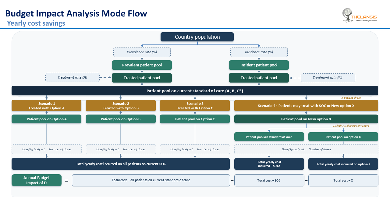
Stripped of therapeutic-area specifics, nearly every budget impact model we build follows the same population-to-cost logic. It’s a seven-step framework designed to isolate the net budget effect of introducing a new treatment option into an existing standard-of-care landscape, and it flexes just as readily to a single head-to-head switch as it does to a crowded, multi-arm comparator landscape.

Step 1: Size the eligible population

Start from the country population and apply prevalence and incidence rates to split out two parallel pools: patients already living with the condition (prevalent) and patients newly diagnosed each year (incident). These are kept separate because they behave differently; prevalent patients may already be on therapy, while incident patients are treatment-naive.

Step 2: Apply treatment rates

Not every diagnosed patient receives active drug therapy. A treatment rate is applied to each pool independently to arrive at the treated patient pool, the population actually eligible to be costed in the model.

Step 3: Map today’s standard of care

The treated pool is allocated across the therapies actually in use today. In a crowded therapeutic area, this can mean several parallel comparator arms rather than one, for example: a chronic condition where current practice spans an intensive procedural option, an advanced cell-based therapy, and long-term supportive management, alongside a newer disease-modifying agent competing for the same patients. Each arm is captured as its own cost stream, with its own dosing logic, like dose per kilogram of body weight and number of doses per year, so per-patient cost is always a bottom-up build, never a single blended number.

Step 4: Model the “new-world” scenario

The treated pool is split again, this time by how much shifts to the new option versus stays on existing standard of care. This split is modeled separately for switch patients (already on therapy, now considering a change) and treatment-naive patients (starting fresh), because the two groups behave very differently: naive patients face no switching friction and typically show higher uptake of a new, often cheaper option, while existing patients are stickier.

Step 5: Cost every arm

Every patient pool, comparator and new intervention alike, is costed using the same three-part logic: unit price × dose per kilogram (scaled to average patient body weight) × number of doses per year. This produces a total yearly cost for each arm of the model.

Step 6: Calculate the budget impact

The core output is deceptively simple: Annual Budget Impact = total cost under the “world without” the new intervention minus total cost under the “world with” it. A positive result is net savings to the payer; a negative result is net additional spend both are valid, expected outputs depending on the scenario.

Step 7: Stress-test it

Every input in Steps 1-5 is an estimate, so the final stage is systematic sensitivity analysis, typically one-way testing on the handful of parameters the model is most exposed to (population size, prevalence, incidence, patient weight, price), visualized as a tornado diagram ranking each parameter by how far it swings the headline result.

Case Example: A Biosimilar Market Entry

1. The Scenario

To make the framework concrete, this case example models the launch of a lower-cost biosimilar competing for share against a single, well-established reference biologic, across five major Western European markets and six related chronic inflammatory indications commonly treated with the same drug class.

This is a familiar payer-facing scenario, and one Thelansis has modeled many times across different biologic classes: once a reference product faces biosimilar competition, every payer wants the same answer before formulary decisions are made, how much could switching, or capturing new patients onto the lower-cost option, actually save, and how much of that saving can they count on?

The commercial logic is simple. If the biosimilar is priced below the originator, every patient who switches, or who starts therapy on the biosimilar rather than the originator, releases a budget that could, in principle, fund additional patients.

2. Applying the Framework: Two Scenarios

The model runs the seven-step framework twice, in parallel, to isolate the budget impact:

• Scenario 1 No biosimilar launch: all eligible patients (naive and switch pools combined) remain on the reference biologic. This is the “world without” baseline.
• Scenario 2 Biosimilar launched: a defined share of both the naive and switch pools moves to the biosimilar, with uptake modeled independently for each group. Naive patients typically show materially higher uptake than switch patients, since starting on the lower-cost option carries none of the friction of moving an already-stable patient off an established therapy.

Annual budget impact = total yearly cost under Scenario 1 (all-reference-biologic) minus [total yearly cost of the remaining reference-biologic patients + total yearly cost of the biosimilar patients] under Scenario 2.

Because list prices for a newly launching biosimilar are rarely known with certainty at the time a forecast is built, the standard approach, and the one used here, is to run the full model across a range of assumed price discounts relative to the reference product, rather than committing to a single point estimate. This example uses three illustrative discount scenarios: 10%, 20%, and 30% below the reference biologic’s list price.

3. Results: Reframing Savings as Additional Patients Treated

A payer-relevant way to present budget impact is not only as a euro figure, but as the number of additional patients who could be treated with the released budget in year one. The tables below show illustrative, anonymized output across the three discount scenarios and the four parameters tested in sensitivity analysis.

➤  10% discount scenario (base case: €25.8M)

➤  20% discount scenario (base case: €51.5M)

➤  30% discount scenario (base case: €77.3M)

Two patterns stand out, and both are exactly what the framework in Section 2 would predict:

• The base-case savings estimate scales up roughly in step with the discount level because price discount is a direct multiplier on every patient-year of switched or naive-captured volume, it doesn’t interact with epidemiology, it just scales the whole result.
• The width of the sensitivity range widens at deeper discounts. The roughly ±10% population swing produces a proportionally similar percentage swing at every discount level, but on a much larger base number so the absolute range in euros is far wider at 30% discount than at 10%. A payer negotiating discount terms is, in effect, also negotiating how much forecast uncertainty they’re willing to absorb.

4. Reading the Sensitivity Pattern

Each discount scenario is also visualized as a tornado diagram, the sensitivity results above, ranked so the parameter with the widest swing sits at the top. Across all three scenarios in this example, the ranking is consistent:

• Number of patients currently treated with the reference biologic: the single biggest lever, because it scales the entire treated population the budget impact is calculated over.
• Prevalence: a meaningful but secondary driver.
• Patient body weight: smaller still, since it affects per-patient dose but not the number of patients.
• Incidence: consistently the smallest driver, because newly diagnosed patients are a much smaller pool than the accumulated prevalent population in a chronic condition, so even a large swing in incidence barely moves the total.

This ordering isn’t a coincidence of the illustrative numbers, it reflects a structural property of the model. Parameters that scale linearly across the entire treated pool (like the share of patients on the reference product) will always dominate a tornado diagram over parameters that only scale a narrower sub-population (like incident-only patients) or only affect per-patient dosing (like body weight). Knowing that in advance tells an analyst, before running a single number, roughly where the sensitivity will concentrate.

5. Market and Indication-Level Granularity

Because the underlying model is built bottom-up by market and by indication, the same base-case output can be sliced multiple ways without rebuilding anything — a direct benefit of the transparent cost-calculator design good-practice guidance favors. Two cuts are typically the most decision-relevant:

• By market: Savings are rarely distributed evenly across a multi-country model, they broadly track population size and current treatment penetration, so the largest market by treated patients contributes disproportionately to the cumulative total, while smaller markets contribute correspondingly less, across all three discount scenarios.
• By indication: Savings also concentrate wherever treated patient volume is highest. In a related set of chronic indications sharing the same drug class, the indication with the largest chronic treated population drives a visibly larger share of total savings than lower-prevalence indications, even though all indications share the same drug and the same discount assumptions.

This granularity is what turns a single headline number into something a market access team can actually act on: it identifies which market-indication combinations are worth prioritizing first for launch sequencing or payer engagement.

6. Validating the Model

Before any client-facing model is finalized, Thelansis cross-checks the structural behavior of the output against internal benchmarks and directional expectations drawn from comparable launches we have modeled across therapeutic areas, confirming that both the size of the effect and the ranking of sensitivity drivers behave the way the underlying epidemiology would predict, before country-specific pricing and access assumptions are layered in.

From Model Output to Deliverable:

A budget impact model is only as useful as the workbook a client actually receives. In practice, Thelansis builds this framework out as a fully linked Excel model, structured across a small number of tabs: raw population and epidemiology inputs (sourced and referenced line by line), a treatment-mix and uptake assumptions tab, a costing engine that applies dosing and unit-price logic per market and per indication, and an outputs/dashboard tab that aggregates everything into the market-, indication-, and scenario-level views shown above.

Every downstream number traces back, through visible formulas, to a sourced input cell, never a hard-coded assumption so a payer, client, or internal reviewer can audit the model without needing the original analyst in the room. A transparent spreadsheet a decision-maker can open and re-run under their own local assumptions will always be more useful, and more defensible, than a more sophisticated model that only its author can interpret.

The Thelansis Approach & Client Value:

A model built this way is more than a headline savings figure, it’s a decision-support tool a client can put in front of a payer with confidence. That’s the standard we hold every budget impact engagement to.

What clients get from working with Thelansis

• A defensible, auditable model: Every output traces to a sourced input, no numbers a client can’t explain if a payer pushes back.
• Launch sequencing built in: Market- and indication-level granularity tells a commercial team where budget impact and payer receptivity is likely to be strongest first, so scarce launch resources go where they’ll land best.
• A pre-built answer to the pricing conversation: Presenting savings across a discount range, rather than a single number, gives a negotiating team a ready answer to “what if we price at X% instead of Y%”, almost always the payer’s first follow-up question.
• Foresight into payer scrutiny: Knowing in advance that patient volume, not epidemiology is the parameter payers are most likely to challenge means a negotiating team can pre-empt that discussion with current market-share data, rather than over-investing in refining estimates that move the result comparatively little.
• A stronger access narrative: Reframing budget impact as a number of additional patients who could be treated is often the more persuasive framing for a public payer whose mandate is patient access, not cost containment for its own sake.

Limitations and Good-Practice Notes:

A few caveats apply to this class of model generally, and to the example above specifically:

• Price is usually the least certain input and the biggest driver of the result. Running a discount range, as done here, is standard practice when a new entrant’s list price isn’t yet public, but it also means the headline savings figure is, functionally, more a function of the price assumption than anything else in the model.
• A one-year, single-cohort model captures a snapshot, not a trend. Multi-year models that account for cumulative uptake growth, patient turnover, and evolving list prices are a natural extension where the decision being supported spans more than one budget cycle.
• Only direct drug acquisition costs are typically captured in a model of this scope. Administration costs, monitoring, and adverse-event management are usually assumed equivalent across comparator and new-entrant arms unless there’s specific evidence otherwise, a simplifying assumption that should always be stated explicitly, not left implicit.

Conclusion:

Budget impact analysis rewards a particular kind of rigor, not analytical cleverness, but traceability. The seven-step Thelansis framework: population, treatment rate, comparator mix, new-world uptake, costing, budget impact, sensitivity is deliberately simple precisely because that simplicity is what makes a model auditable, defensible, and reusable across therapeutic areas as different as a chronic biosimilar switch and a multi-arm rare-disease treatment landscape.

This case example shows that framework doing its job: turning a set of population and pricing assumptions into a market-by-market, indication-by-indication forecast that a commercial team can act on and a payer can independently verify. That, in the end, is the entire point of a budget impact model, and it’s the standard every Thelansis engagement is built to meet.